Strategy Objects & Slippage¶

simple-back backtests might be too optimistic, in reality you will hardly ever purchase securities at the exact open or close price. To help with this, you can use slippage. But first, let’s turn our backtest from before into its own object.

[1]:

from simple_back.strategy import Strategy

Strategy Object for our Moving Average from Before¶

[2]:

class MAStrategy(Strategy):
    def __init__(self, ticker, ma_days, cool_days=60, no_log=False):
        self.ticker = ticker
        self.ma_days = ma_days # length of the MA
        self.cool_days = cool_days # length of the cooldown period
        self.no_log = no_log

    @property
    def name(self):
        return f"{self.ticker} - MA ({self.ma_days} days), CD ({self.cool_days} days)"

    def run(self, day, event, b):
        if event == 'open':
            ma = b.prices[self.ticker,-self.ma_days:]['close'].mean()
            b.add_metric('Price', b.price(self.ticker))
            b.add_metric(f'MA ({self.ma_days} Days)', ma)

            last_pos_date = b.portfolio.attr('date')
            if last_pos_date is None:
                date_diff = self.cool_days
            else:
                date_diff = (day - last_pos_date).days

            if date_diff >= self.cool_days and b.portfolio.total_value >= 0:
                if b.price(self.ticker) > ma:
                    if not b.portfolio[self.ticker].long: # check if we already are long
                        if not self.no_log:
                            b.log(f'long {self.ticker}')
                        b.portfolio[self.ticker].short.liquidate() # liquidate any/all short positions
                        b.long(self.ticker, percent=1) # long

                if b.price(self.ticker) < ma:
                    if not b.portfolio[self.ticker].short: # check if we already are short
                        if not self.no_log:
                            b.log(f'short {self.ticker}')
                        b.portfolio[self.ticker].long.liquidate() # liquidate any/all long positions
                        b.short(self.ticker, percent=1) # short

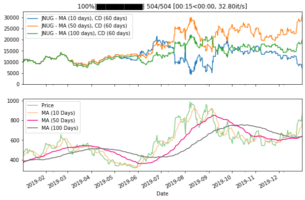
Now we can use our strategy from before, but can easily compare how it performs with different tickers, MA lengths or different lengths of the cooldown period.

Running Strategies¶

We can run several strategies without iterating using run.

[3]:

from simple_back.backtester import BacktesterBuilder

builder = (
   BacktesterBuilder()
   .balance(10_000)
   .calendar('NYSE')
   .strategies([
       MAStrategy('JNUG',10),
       MAStrategy('JNUG',50),
       MAStrategy('JNUG',100),
    ]) # strategies to run
   .live_progress() # show a progress bar using tqdm
   .live_plot() # we assume we are running this in a Jupyter Notebook
)

[4]:

bt = builder.build()
bt['2019-1-1':'2020-1-1'].run()

JNUG - MA (10 days), CD (60 days)
		log
date	event
2019-01-02 00:00:00	open	long JNUG
2019-03-04 00:00:00	open	short JNUG
2019-05-08 00:00:00	open	long JNUG
2019-07-09 00:00:00	open	short JNUG
2019-09-17 00:00:00	open	long JNUG
2019-11-22 00:00:00	open	short JNUG

JNUG - MA (50 days), CD (60 days)
		log
date	event
2019-01-02 00:00:00	open	long JNUG
2019-03-04 00:00:00	open	short JNUG
2019-06-03 00:00:00	open	long JNUG
2019-08-19 00:00:00	open	short JNUG
2019-10-25 00:00:00	open	long JNUG

JNUG - MA (100 days), CD (60 days)
		log
date	event
2019-01-02 00:00:00	open	long JNUG
2019-03-07 00:00:00	open	short JNUG
2019-06-05 00:00:00	open	long JNUG
2019-09-10 00:00:00	open	short JNUG
2019-12-03 00:00:00	open	long JNUG

Note:

The dataframes below the plot are generated because we now use .log instead of .add_line as the lines of the different backtests would just overlap.

Slippage¶

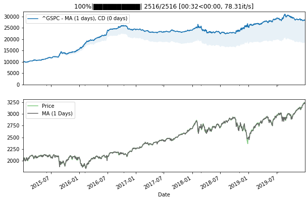
The more often trades are executed, the more slippage can become a problem. To visualize this, we can simply use .slippage, now with just one strategy.

Note:

Slippage is set to 0.05% per default, which is the same quantopian uses for US Equities (as of 06-2020).

[5]:

bt = builder.strategies([MAStrategy('JNUG',10)]).no_live_progress().no_live_plot().slippage().build()
bt['2019-1-1':'2020-1-1'].run()

This is not a display error, we just trade so little that slippage is hardly noticeable. To get the exact difference, we can look at the summary again, where we can spot that slippage only causes 1% less in total return.

[6]:

bt.summary

[6]:

	Max Drawdown (%)	Annual Return	Portfolio Value (Last Value)	Total Value (Last Value)	Total Return (%) (Last Value)	Daily Profit/Loss (Last Value)
Backtest
JNUG - MA (10 days), CD (60 days) (lower bound)	-80.370444	0.767375	7386.879668	7686.275872	-23.137241	88.579424
JNUG - MA (10 days), CD (60 days)	-80.125384	0.775959	7410.557799	7771.721211	-22.282788	88.535156

But what if we trade more often? Let’s set the cooldown period to 0, MA to 1 and test over a longer period.

[7]:

bt = builder.strategies([MAStrategy('^GSPC',1,0,no_log=True)]).slippage().build()
bt['2015-1-1':'2020-1-1'].run()

[8]:

bt.summary

[8]:

	Max Drawdown (%)	Annual Return	Portfolio Value (Last Value)	Total Value (Last Value)	Total Return (%) (Last Value)	Daily Profit/Loss (Last Value)
Backtest
^GSPC - MA (1 days), CD (0 days) (lower bound)	-27.266620	1.128103	15973.746320	18256.626462	82.566265	-124.650650
^GSPC - MA (1 days), CD (0 days)	-16.081719	1.230159	25596.638672	28135.337158	181.353372	-173.681641