Creating a Simple Strategy
In this tutorial, we will build a crossover strategy that exclusively buys and sells JNUG. It will enter a long position whenever the price goes above its 20-day MA and enter a short position when it goes below.
Building a Backtest
Use .BacktesterBuilder to configure and create a .Backtester object.
[2]:
from simple_back.backtester import BacktesterBuilder

builder = (
   BacktesterBuilder()
   .name('JNUG 20-Day Crossover')
   .balance(10_000)
   .calendar('NYSE')
   .compare(['JNUG']) # strategies to compare with
   .live_progress() # show a progress bar using tqdm
   .live_plot() # we assume we are running this in a Jupyter Notebook
)
Running the Backtest
We can now treat the bt object like an iterator with a date index.
[3]:
bt = builder.build()
for day, event, b in bt['2019-1-1':'2020-1-1']:
    pass
    # code here will be called
    # on 'open' and 'close' events on trading days

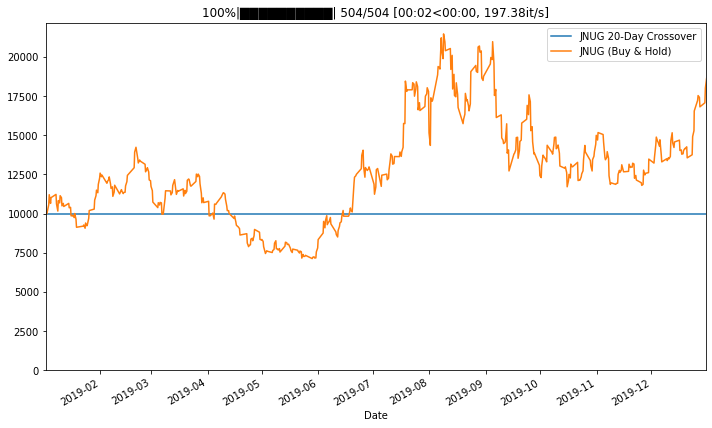
Note that we wrote .compare(['JNUG']) before so we could compare our strategy to just buying and holding JNUG. Because we do not do anything so far, the JNUG 20-Day Crossover strategy results in a flat line.
Note:
.BacktesterBuilder.compare normally only accepts a list of .Strategy objects, but for each string that is passed, it automatically creates a .BuyAndHold strategy for the symbol represented by the string.
Creating a Strategy
We are now ready to create the strategy. Although not necessary for this strategy, we will only act on market open by checking that event == 'open'
We then calculate the 20-day moving average of JNUGs close prices.
[4]:
bt = builder.no_live_plot().build()
for day, event, b in bt['2019-1-1':'2020-1-1']:
    if event == 'open':
        jnug_ma = b.prices['JNUG',-20:]['close'].mean()
100%|██████████| 504/504 [00:02<00:00, 179.12it/s]
Note:
The second indexer of b.prices (implemented in .DailyPriceProvider) can be a date range or single date that allows you to use int, dateutil.relativedelta.relativedelta or datetime.date values.
We can check if the current price is above or below the moving average using b.price('JNUG').
[5]:
bt = builder.no_live_plot().build()
for day, event, b in bt['2019-1-1':'2020-1-1']:
    if event == 'open':
        jnug_ma = b.prices['JNUG',-20:]['close'].mean()
        if b.price('JNUG') > jnug_ma:
            pass
            # price is above MA
        if b.price('JNUG') < jnug_ma:
            pass
            # price is below MA
100%|██████████| 504/504 [00:01<00:00, 285.25it/s]
Now we should only need to buy when the price is above, and sell when the price is below the MA.
[6]:
bt = builder.no_live_plot().build()
for day, event, b in bt['2019-1-1':'2020-1-1']:
    if event == 'open':
        jnug_ma = b.prices['JNUG',-20:]['close'].mean()
        if b.price('JNUG') > jnug_ma:
            b.long('JNUG', percent=1) # as percent of total value
        if b.price('JNUG') < jnug_ma:
            b.short('JNUG', percent=1) # as percent of total value
1%| | 3/504 [00:00<00:06, 79.13it/s]
InsufficientCapitalError:
                        not enough capital available:
                        ordered 1 * 10563.648455632008
                        with only 449.31090733719975 available
But as you might already have expected, this fails with an .InsufficientCapitalError This is because we repeatedly try to invest 100% of our assets into JNUG, even when we already hold JNUG shares.
Note:
.Backtester.long and .Backtester.short allow for use of the following arguments: percent: order as percent of total value; percent_available: order as percent of the available cash; absolute: order as absolute cash value; nshares: order as number of shares.
To fix the previous error we now check if the corresponding positions are already in our portfolio, and liquidate positions of the wrong kind. We liquidate long positions before we go short and vice versa:
[7]:
bt = builder.build()
for day, event, b in bt['2019-1-1':'2020-1-1']:
    if event == 'open':
        jnug_ma = b.prices['JNUG',-20:]['close'].mean()

        if b.price('JNUG') > jnug_ma:
            if not b.portfolio['JNUG'].long: # check if we already are long JNUG
                b.portfolio['JNUG'].short.liquidate() # liquidate any/all short JNUG positions
                b.long('JNUG', percent=1) # long JNUG

        if b.price('JNUG') < jnug_ma:
            if not b.portfolio['JNUG'].short: # check if we already are short JNUG
                b.portfolio['JNUG'].long.liquidate() # liquidate any/all long JNUG positions
                b.short('JNUG', percent=1) # short JNUG

While running, the .Backtester.portfolio (with the shorthand .Backtester.pf) object keeps track of positions. If we hold a position at the very end of the backtest, it will remain in this object. .Backtester.portfolio.df holds a dataframe of said positions.
[9]:
b.portfolio.df # shorthand: b.pf.df
[9]:
| date | event | initial_value | nshares | order_type | price | profit_loss_abs | profit_loss_pct | start_price | symbol | value | value_pershare | |
|---|---|---|---|---|---|---|---|---|---|---|---|---|
| 0 | 2019-12-24 | open | 4238.278808 | 6.0 | long | 832.202148 | 754.934082 | 0.178123 | 706.379801 | JNUG | 4993.212891 | 832.202148 |
Inspecting Metrics
Now that our Backtest is complete, we can use .Backtester.metrics and .Backtester.summary to get more details. Both of these will return DataFrames.
Metrics
[10]:
bt.metrics
[10]:
| Max Drawdown (%) | Annual Return | Portfolio Value | Total Value | Total Return (%) | Daily Profit/Loss | |||
|---|---|---|---|---|---|---|---|---|
| Backtest | Date | Event | ||||||
| JNUG 20-Day Crossover | 2019-01-02 | open | -71.121124 | 0.525525 | 0.000000 | 10000.000000 | 0.000000 | 0.000000 |
| close | -71.121124 | 0.525525 | 9696.819855 | 10146.130762 | 1.461308 | 0.000000 | ||
| 2019-01-03 | open | -71.121124 | 0.525525 | 10114.337548 | 10563.648456 | 5.636485 | 563.648456 | |
| close | -71.121124 | 0.525525 | 10751.050232 | 11200.361139 | 12.003611 | 1054.230377 | ||
| 2019-01-04 | open | -71.121124 | 0.525525 | 10197.839717 | 10647.150624 | 6.471506 | 83.502169 | |
| ... | ... | ... | ... | ... | ... | ... | ... | ... |
| JNUG (Buy & Hold) | 2019-12-27 | close | -49.921226 | 1.799052 | 16358.200195 | 16807.511103 | 68.075111 | -718.145142 |
| 2019-12-30 | open | -49.921226 | 1.799052 | 16615.727700 | 17065.038607 | 70.650386 | -343.369146 | |
| close | -49.921226 | 1.799052 | 17553.713379 | 18003.024286 | 80.030243 | 1195.513184 | ||
| 2019-12-31 | open | -49.921226 | 1.799052 | 18221.607392 | 18670.918299 | 86.709183 | 1605.879692 | |
| close | -49.921226 | 1.799052 | 17476.245117 | 17925.556025 | 79.255560 | -77.468262 |
1008 rows × 6 columns
Summary
[11]:
bt.summary
[11]:
| Max Drawdown (%) | Annual Return | Portfolio Value (Last Value) | Total Value (Last Value) | Total Return (%) (Last Value) | Daily Profit/Loss (Last Value) | |
|---|---|---|---|---|---|---|
| Backtest | ||||||
| JNUG 20-Day Crossover | -71.121124 | 0.525525 | 4993.212891 | 5276.118290 | -47.238817 | -22.133789 |
| JNUG (Buy & Hold) | -49.921226 | 1.799052 | 17476.245117 | 17925.556025 | 79.255560 | -77.468262 |
Strategies
You can also use .Backtester.strategies which returns a .StrategySequence, with their own .Backtester.metrics and .Backtester.summary.
[12]:
bt.strategies['JNUG 20-Day Crossover'].metrics
[12]:
| Max Drawdown (%) | Annual Return | Portfolio Value | Total Value | Total Return (%) | Daily Profit/Loss | |||
|---|---|---|---|---|---|---|---|---|
| Backtest | Date | Event | ||||||
| JNUG 20-Day Crossover | 2019-01-02 | open | -71.121124 | 0.525525 | 0.000000 | 10000.000000 | 0.000000 | 0.000000 |
| close | -71.121124 | 0.525525 | 9696.819855 | 10146.130762 | 1.461308 | 0.000000 | ||
| 2019-01-03 | open | -71.121124 | 0.525525 | 10114.337548 | 10563.648456 | 5.636485 | 563.648456 | |
| close | -71.121124 | 0.525525 | 10751.050232 | 11200.361139 | 12.003611 | 1054.230377 | ||
| 2019-01-04 | open | -71.121124 | 0.525525 | 10197.839717 | 10647.150624 | 6.471506 | 83.502169 | |
| ... | ... | ... | ... | ... | ... | ... | ... | ... |
| JNUG (Buy & Hold) | 2019-12-27 | close | -49.921226 | 1.799052 | 16358.200195 | 16807.511103 | 68.075111 | -718.145142 |
| 2019-12-30 | open | -49.921226 | 1.799052 | 16615.727700 | 17065.038607 | 70.650386 | -343.369146 | |
| close | -49.921226 | 1.799052 | 17553.713379 | 18003.024286 | 80.030243 | 1195.513184 | ||
| 2019-12-31 | open | -49.921226 | 1.799052 | 18221.607392 | 18670.918299 | 86.709183 | 1605.879692 | |
| close | -49.921226 | 1.799052 | 17476.245117 | 17925.556025 | 79.255560 | -77.468262 |
1008 rows × 6 columns
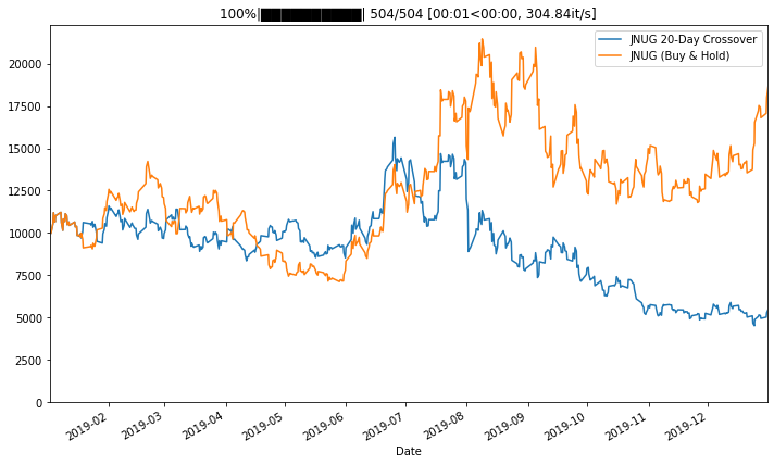
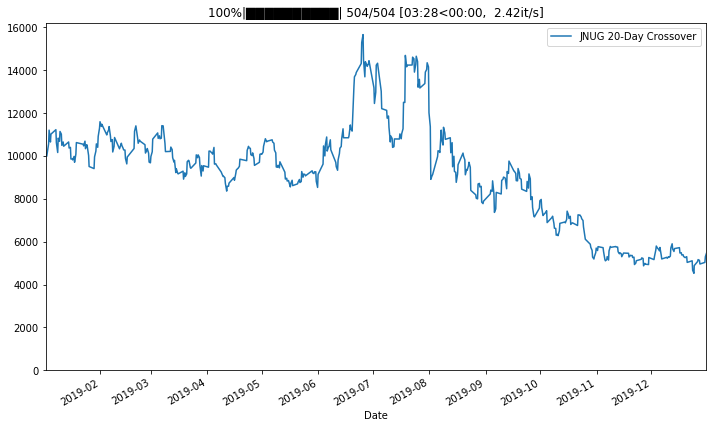
The advantage of using using .StrategySequence is that we can also use it for plotting.
[13]:
bt.strategies[0].show()
